Bayes, Regression, and the Red Sox (but mostly Bayes)

WARNING: Math heavy post.

Let's say that we have a hypothetical Major League team that has started the season 2-10. Say we want to see how likely it is that a team that goes 2-10 is still a .500 team. If you've taken any statistics courses, you may be familiar with hypothesis testing where you formulate a null hypothesis that the team is a .500 team, and then calculate the probability that they would go 2-10 by chance. You would then see that a .500 team will go 2-10 (or worse) over a 12 game span less than 2% of the time, and you'd probably reject your null hypothesis, depending on how high you set your significance level.

This does not, however, tell you anything about the likelihood that the team actually is a .500 team, only the likelihood that they would perform that badly if they were in fact a .500 team. To address the former issue, we can instead use a Bayesian approach.

To do that, we have to make an assumption about the population that the team is drawn from (in other words, about the spread of talent across all teams in the league). Most teams in MLB fall somewhere in the .400-.600 range (at least in true talent, if not in observed win percentage), so for convenience sake, let's just assume MLB teams follow a normal distribution of talent with a standard deviation of .050 W%.

This is our prior distribution. Once we have that, we can apply Bayes' Theorem:


P(A|B) = P(B|A)*P(A)/P(B)

We want to find the probability of A given B [P(A|B)], which is to say that we want to find the probability that a team drawn from our prior population distribution (u=.500, SD=.050) is actually a .500 (or better) team, given that we have observed that team to go 2-10 over 12 games. To do this, we need to find the probabilities P(B|A), P(A), and P(B).

P(A) is the simplest. This is the probability of a random team drawn from our prior distribution is at least a .500 team, ignoring of what we observed over the 12 game sample. This is just .500, because the population is centered around .500. So, P(A)=.5.

*NOTE-if you want to use a W% other than .500, all you have to do is find the probability of drawing a W% at least that high from the prior distribution, which is trivial when the prior distribution is normal since that is a common computer function. If you don't have a program that can calculate normal distribution probabilities, you can use an online tool.

P(B) is a bit more difficult. This is the probability that we observe a random team drawn from our prior distribution to go 2-10 over 12 games. This would be simple to calculate for any one team if we already know its true W%, but we need to know the average probability for all possible teams we could draw from our prior distribution. This will require a bit of calculus.

For any one team with a known true W% (p), the probability of going 2-10 is:

( 12! / (2! * 10!) ) * p^2 * (1-p)^10

where 12 represents the number of total games, 2 the number of wins, and 10 the number of losses. We need to find the average value of that formula across the entire prior distribution.

To do this, we utilize the same principle as a weighted average. In this case, the weight given to each possible value of p is represented by the probability density function of the prior distribution. So, for example, the odds of a .400 team going 2-10 are about 6.4%, and that 6.4% gets weighted by the quantity f(p), where f(p) is the pdf for our prior normal distribution. We repeat this for each possible value of p, add up the weighted terms, and then divide by the sum of the weights. As you have probably guessed, this means taking the definite integral (from p=0 to p=1) of the probabilities weighted by f(p):

INTEGRAL(f(p) * ( ( 12! / (2! * 10!) ) * p^2 * (1-p)^10 ) dp)

f(p) is just the normal distribution pdf, which is:

f(p) = e^((-((x-u)^2))/(2*VAR))/(sqrt(2*Pi*VAR)) ; u=.5, VAR=.05^2=.0025

As fun as it sounds to go ahead and do that by hand, we'll just let computers do this part for us too, using an online definite integral calculator. You can copy and paste this into the function field if you want to try it for yourself:

((12!/(2!*10!))*exp((-((x-.5)^2))/(2*.0025))*(x^2*(1-x)^10)/(sqrt(2*3.14159*.0025)))

or, more generally, if you want to play around with different records or different means and variances for the prior normal distribution:

(((W+L)!/(W!*L!))*exp((-((x-u)^2))/(2*VAR))*(x^W*(1-x)^L)/(sqrt(2*Pi*VAR)))

Integrating that from 0 to 1, we get a total value of .020. Remember that we still have to divide by the total sum of the weights to find the weighted average, but since that is just F(p), or the cumulative distribution function of the prior distribution, it is equal to one by definition. Therefore, P(B) = .02.

Finally, we have to calculate P(B|A). This is the probability of observing a 2-10 record, given that we are drawing a random team from the prior distribution that fulfills condition A, which is that the team has at least a .500 true W%. This is done very similarly to finding P(B) above, except we are only considering values of p>.5.

Start by calculating the same definite integral as before, but from .5 to 1 instead of from 0 to 1 (this is done by simply changing a textbox below the formula). This gives a value of .0045. That is the weighted sum of all the probabilities; to turn the weighted sum into an average, we still have to divide by the sum of all the weights, which in this case is .5 (this is the cdf F(p) from .5 to 1). Dividing .0045 by .5, we get .009. This is P(B|A).

P(A)=.5
P(B) = .02
P(B|A) = .009

P(A|B) = .009*.5/.02 = .22

The probability of a team that goes 2-10 being at least a true talent .500 team is about 22% (assuming our prior distribution is fairly accurate). As you can see, this is pretty far from what one might conclude from using the hypothesis test to reject the null hypothesis that the team is a .500 team. This is why it is important not to misconstrue the meaning of the hypothesis test. The hypothesis test only tells you a very specific thing, which is how likely or unlikely the observed result is if you assume the null hypothesis to be true. Rejecting the null hypothesis on this basis does not necessarily mean the null hypothesis is unlikely; that depends on the prior distribution of possible hypotheses that exist. Considering potential prior distributions allows us to make more relevant estimates and conclusions about the likelihood of the null hypothesis.

Another advantage of the Bayesian approach is that it gives us a full posterior distribution of possible results. For example, when we observe a 2-10 team, we can not only estimate the odds that it is a true .500 team, but also the odds that it is a true .550 team, or .600 team, or whatever. Also, since we have a full distribution of likelihoods, we can also figure out the expected value.

The posterior distribution of possible true talent W% for a team that is observed to go 2-10 is represented by the product we integrated earlier:

(((W+L)!/(W!*L!))*exp((-((x-u)^2))/(2*VAR))*(x^W*(1-x)^L)/(sqrt(2*Pi*VAR)))

We find the expected value of that function the same way we found the average value of the above probabilities. This time, we want to find the average value of x (or p, as we were calling it before), so we weight each value of x by the above function, and then divide by the sum of the weights. For the numerator, this means integrating the above function multiplied by x:

x * (((W+L)!/(W!*L!))*exp((-((x-u)^2))/(2*VAR))*(x^W*(1-x)^L)/(sqrt(2*Pi*VAR)))

The denominator is just the summation of the function not multiplied by x, which we already did above (it is the same thing as the P(B) above, or .020).

Plugging this into the definite integral calculator, we get:

0.009442586/0.020355243 = 0.464

So a team that goes 2-10 over 12 games will be, on average, about a .464 team (again, assuming our prior distribution is accurate).

As a shortcut for the above calculations, one can also use regression to the mean to estimate the expected value of the team's true W%. This is done by finding the point where random variance in the observed record equals the variance of talent in the population. We know the standard deviation of talent in the population, using our assumed prior, is .050 wins per game. The random variance in the observed record is n*p*(1-p), where n is the number of games and p is the teams' true W%. Since p mostly stays around .5, this approximately equal to n*.25 (it's actually about n*.2475, but the difference is minimal). When you have 100 observed games, the random variance will be 100*.25 = 25. The variance of talent will be (100*.05)^2 = 25. Therefore, after 100 games, the variance due to random variation will equal the variance of talent in the population.

At this point, we would regress exactly 50% to the mean to estimate the expected value of a team's true W%. This is the same as adding 100 games of league average performance to a team's observed record. This also works after any observed number of games. To estimate our 2-10 team's true W% with regression to the mean, we would add 50 wins and 50 losses to the observed record and get an expected W% of 52/112 = .464. How well regression to the mean approximates Bayesian probability depends on the prior distribution you choose, but in this case, it works very well (rounds to the same thousandths place).

This is all done assuming a prior that presumes nothing about the team in question other than the fact that it comes from a distribution of teams roughly like that we observe in MLB. What if, in addition to knowing the 2-10 team comes from MLB, we also know that the team employs several really good players and that we believe them to be one of the most talented teams in the league? We can adjust the prior for that information as well. Our prior distribution, after accounting for the amount of talent we believe to be on the team, might have a mean of .590 instead of .500. Let's say that we assume a normal distribution with a mean of .590 and a SD of .030 for our prior. Now we get an expected W%, after observing the team go 2-10, of .572. In this case, the absymal 12 game observed sample dropped our expectations for the team going forward from .590 to .572. Of course, this all depends on what prior you assume, but as long as you make reasonable assumptions, your estimate should give you a decent idea. Continue Reading...

Optimistic Projections.

UPDATE: The table in the article has been updated with actual 2011 wOBAs for each player, along with actual 2011 PAs. An aggregate line has been added with the combined projected and actual wOBAs weighted by actual 2011 PAs. Also, in light of Mike's response below regarding the handling of intentional walks in their projections, it is possible the RotoChamp wOBA values are artifically-inflated, so the difference between the average Roto projection and the actual might not be meaningful.

While looking through the projections posted at FanGraphs, I noticed that some of the RotoChamp projections seem a bit optimistic. For example, Jim Thome is projected with a .419 wOBA. Thome had a good year last year, putting up a .437 wOBA over 340 PA, but he's also 40 years old, and even with a potential HOF career behind him, his career wOBA is only .407.

This looks like a simple case of under-regressing 2010 performance and not enough weight given to past performance. However, other optimistic projections fall out of this pattern. For example, Albert Pujols is projected with a .449 wOBA, higher even than his career .434 mark despite Albert now being on the wrong side of 30 (it appears the wOBA projections may not remove IBB, so Albert's career wOBA with his IBBs counted as nIBBs would be .444; closer to his projection, but still lower). Albert's 2010 performance, however, does not seem to be driving the high projection; he hit only .420 last year.

Does RotoChamp see something important in projections like these, or is the optimism misplaced? I find 20 different players listed in both the Marcel and RotoChamp projections who are projected at least .030 points wOBA higher by RotoChamp than Marcel. They are:

Name	Age	Rel	Marcel	RotoChamp	diff	2011 PA	2011 wOBA
Jim Thome	41	0.81	0.360	0.419	0.059	324	0.362
Dan Johnson	32	0.4	0.327	0.381	0.054	91	0.181
Jose Bautista	31	0.84	0.362	0.408	0.046	655	0.441
Brandon Allen	25	0.38	0.321	0.367	0.046	195	0.286
Ramon Castro	35	0.6	0.319	0.361	0.042	75	0.332
Magglio Ordonez	37	0.83	0.345	0.386	0.041	357	0.283
Ryan Hanigan	31	0.69	0.329	0.370	0.041	304	0.320
Chipper Jones	39	0.83	0.353	0.393	0.04	512	0.345
Jorge Posada	40	0.79	0.341	0.381	0.04	387	0.309
Matt Diaz	33	0.74	0.330	0.367	0.037	268	0.280
Andruw Jones	34	0.75	0.323	0.360	0.037	222	0.371
Albert Pujols	31	0.87	0.414	0.449	0.035	651	0.385
David Ortiz	36	0.85	0.347	0.382	0.035	605	0.405
Jason Giambi	40	0.78	0.326	0.359	0.033	152	0.407
Matt Treanor	35	0.64	0.279	0.312	0.033	242	0.291
Miguel Cabrera	28	0.87	0.390	0.422	0.032	688	0.436
Chase Utley	33	0.86	0.370	0.401	0.031	454	0.344
Aubrey Huff	35	0.87	0.345	0.376	0.031	579	0.294
Jed Lowrie	27	0.65	0.336	0.367	0.031	341	0.297
Manny Ramirez	39	0.81	0.371	0.401	0.03	17	0.052
						TOTAL PA
weighted average			0.354	0.392		7119	0.353

This does not include prospects who have not appeared in the Majors, such as Brandon Belt, who RotoChamp likes a lot (.385 projected wOBA). Technically, Marcel projects these players with a league average wOBA, so they could be included, but whether or not RotoChamp's prospect insights add value is a separate issue than what I am looking at here. Other than Brandon Allen, these players all have fairly established Major League track records with plenty of data for a projection system to work with, and RotoChamp is still seeing them very differently from Marcel.

The test here is simple. At the end of the year, will Marcel's or RotoChamp's estimates for these 20 players be better? Additionally, will this group signicantly outperform its Marcel projections, even if they still end up closer to Marcel than RotoChamp? After all, RotoChamp could be finding something that Marcel is underselling in these players and still be over-weighting that insight to end up with overly optimistic projections.

Most of the players on the list are in their 30s or 40s (all except Miguel Cabrera, Jed Lowrie, and Brandon Allen). Their average age is 34. Many, like Thome, Jose Bautista, and Andruw Jones are coming off big 2010 seasons, while some, like Albert and Manny Ramirez, are big names projected for bigger numbers than their 2010s would indicate. Continue Reading...

Primary Position Table for MySQL (a.k.a. the lamest Christmas present you will ever receive)

As indicated by the notice in the margin, my computer died recently, so I have been rebuilding my databases the past few days. While I was at it, I figured this was as good a time as any to finally build a primary position table rather than keep writing various position requisites into each query whenever I need it. I also figured this may be of use to someone else as well, so I'm publishing the query I wrote here as my Christmas gift to you (if you would like to use this query but do not celebrate Christmas, feel free to classify this gift accordingly; if you would like something a little less esoteric for Christmas, well, that's what family and friends are for).

Merry Christmas (link to query text)

A few notes on this query:

• It is written for MySQL. I don't know how well it would adapt to other programs.


• It is written for use with the Baseball-Databank. bbdatabank is the name of my database; if you have named yours something different, change occurrences of "bbdatabank.*" accordingly.


• This query creates a table that lists each defensive position played by a player and indicates whether the position is that player's primary position. The line "CREATE TABLE bbdatabank.prim_pos AS" (line 10) is currently commented so that the query will not create the table but display the results instead. You can run it as is to check the output, or you can un-comment that line (delete the "#" in front of it) to create the table in the bbdatabank database.


• I classified both corner OF spots as one position (for example, Ty Cobb's primary position is listed as CF, while Hank Aaron's is corner OF). I do this because if a player has 100 games each at LF and RF, and 105 G at CF, I consider him primarily a corner OF and not a center fielder, but you can change this with some minor tweaks to the code if you want.


• For years prior to and including 1955, OF games are broken down by position in a separate table of the Baseball-Databank db, so to get games split out between LF/RF/CF, you need to use two different tables to get defensive games. However, 1954 and 1955 have OF games split out by individual position in the main fielding table as well, so you need to exclude those years from one table or the other to avoid double counting. I chose to just use the fieldingOF table in its entirety and cut 1954-55 from the main fielding table, but you can switch that if you want. There are some minor discrepancies between the two tables, but it shouldn't make a huge difference (at least not from any of the entries I have looked at).


• I apologize if the query looks much longer and nastier than it needs to. It could probably be written more concisely, especially if I used joins, but I try to avoid using joins on large tables like this if I can help it, because using unions and variables to do the same thing runs much, much faster on my computer. Speaking of which, this query actually has multiple statements that need to be run (the various statements at the beginning that set the initial variable values, and then the one long query), so it would be useful to run this as a script. That is not a problem in the new MySQL Workbench or the command line, but if you are still using the old Query Browser, that might not work. If you are using the old Query Browser, all you have to do is run each of those SET statements on its own before running the main query (all in the same tab). I haven't tested the query without running those statements first to check whether the results are still accurate, so I guess it might work anyway, but I strongly recommend using them.

The method for determining a player's primary position has two steps. First, each position is categorized as follows:

-P: Pithcer
-C: Catcher
-off_IF: 1B, DH (I know DH is not an infield position; I just wanted to classify these two positions together, and this is what I called it. You can change it if it bothers you)
-def_IF: 2B, 3B, SS
-OF: cOF, CF (remember that I combine LF and RF into cOF)

I total a player's games in each category and used that to determine a player's primary category. Then, I looked at the number of games at each position in each category and determine the primary position within each category. The primary position in the primary category is the player's overall primary position. For example, let's look at Willie Bloomquist:

DH- 21 G; 1B-21 G; 2B-106 G; 3B- 121 G; SS-150 G; CF-186 G; cOF-37 G

That gives us category totals of:

P: 0
C: 0
off_IF: 58
def_IF: 377
OF: 295

Here, we see that Willie's primary category is def_IF. That means his primary position has to come from this category. Of those positions (2B, 3B, SS), he has the most games as SS, so that is his primary position, even though he has more games at cOF than at SS.

The fields generated for this table are:

• playerID


• prim_pos: 0 if the position is not the player's primary position, 1 if it is


• pos: defensive position


• cat: the category the position is classified in, as described above


• G: defensive games


• tot: combined defensive games at all positions


• cat_tot: combined defensive games at all positions in that category


• maxP: 0 if the position is not the primary position for that category (Pos with max games in that category only), 1 if it is


• prim_cat: 0 if the category is not the primary category, 1 if it is


• percPos: the percentage of total defensive games that are at that position (G/tot)


• percCat: the percentage of total defensive games that are in that category (cat_tot/tot)


• percP_C: the percentage of defensive games in that category that are at that position (G/cat_tot)

Hacking the Hack:

Splitting up cOF into LF and RF: Perhaps you don't like that I combine LF and RF into one position. Splitting them back up shouldn't be too much trouble. Where pos is defined as "if(pos='LF','cOF',if(pos='RF','cOF',pos))", (such as in line 108, but there are other places that will need to be changed as well), change that to just "pos" (no quotes). For example:


(SELECT playerID, if(pos='LF','cOF',if(pos='RF','cOF',pos)) as pos
,sum(if(yearID<=1955 and pos regexp 'F$',0,G)) as G
,if(pos='2b' or pos='3b' or pos='ss','def_IF'
,if(pos='1b' or pos='DH','off_IF'
,if(pos='P','P' ,if(pos regexp 'F$','OF','C')))) as cat
from bbdatabank.fielding
where pos!='OF'
group by playerID, if(pos='LF','cOF',if(pos='RF','cOF',pos))

would become


(SELECT playerID, pos
,sum(if(yearID<=1955 and pos regexp 'F$',0,G)) as G
,if(pos='2b' or pos='3b' or pos='ss','def_IF'
,if(pos='1b' or pos='DH','off_IF'
,if(pos='P','P' ,if(pos regexp 'F$','OF','C')))) as cat
from bbdatabank.fielding
where pos!='OF'
group by playerID, pos

I think there are 4 instances where that has to be changed (the above two changes at lines 108 and 116, plus two more at 137/145).

Also, you will need to change the query of the fieldingOF table to split cOF into LF and RF:


UNION ALL

SELECT playerID, 'cOF' as pos, sum(Glf+Grf) as G, 'OF' as cat
from bbdatabank.fieldingof
group by playerID


should become:


UNION ALL

SELECT playerID, 'LF' as pos, sum(Glf) as G, 'OF' as cat
from bbdatabank.fieldingof
group by playerID

UNION ALL

SELECT playerID, 'RF' as pos, sum(Grf) as G, 'OF' as cat
from bbdatabank.fieldingof
group by playerID


The above change will need to be done in two places.

These changes will make it so the 100/105/100 split for OF games at LF/CF/RF selects CF as the primary position. It would also be possible to keep the corner OF designation but still specify LF or RF as a primary overall position. You would want to create a second type of category just for corner OF. You could do this by copying and pasting the appropriate part of the code and then editing the appropriate lines, but this is going to require knowing which part of the code adds the new columns for "cat" and "pos". This would probably be more straightforward if the code used joins, but it doesn't (sorry). I would actually prefer to do it this way, but I was tired of writing this query and it is not that important to me to split up LF and RF, so I didn't get to it. If I do it sometime later, I'll update the linked query text.

Changing the groupings of position categories: Don't like how I chose to group the positions? Not a problem. The section you need to change is:


if(pos='2b' or pos='3b' or pos='ss','def_IF'
,if(pos='1b' or pos='DH','off_IF'
,if(pos='P','P'
,if(pos regexp 'F$','OF','C')))) as cat


I believe this appears at lines 45, 59, 79, 110, and 139 (assuming you haven't added or removed lines editing other things, of course). For each occurrence, edit that statement to fit your liking (just make sure you edit each occurrence to the same thing). For example, you can move 1B into one IF group with 2B, 3B, and SS and leave DH as its own separate group, or group the positions into corner positions and up the middle positions. If you want to add more groups, just add a new line to the if statement just like the others, and add a close-parenthesis at the end next to the others. If you want to delete a category, make sure to also delete a close-parenthesis. The catcher category right now is just left as whatever is leftover after the other positions are assigned, but you can add a separate line for the catcher class if you want. For example, you might do this:


if(pos='2b' or pos='ss' or pos='c','middle_IF'
,if(pos='1b' or pos='3b','corner_IF'
,if(pos regexp 'F$','OF'
,if(pos='P','P'
,if(pos='DH','DH',''))))) as cat


Note that when I used an explicit if statement for each individual category (i.e. no just assigning the leftovers to a category, like I did with catchers above), I still have to end with ",''" before the close-parentheses. You need something there between the last comma and the series of close-parentheses for the query to run.

IMPORTANT: the fielding table has entries for both individual outfield positions and for combined OF totals. If you don't do something about this, OF games will be double counted, so the following line appears near each of the category definition occurrences:


where pos!='LF' and pos!='RF' and pos!='CF'


This is because I am classifying all OF positions in the same category, so I just use the OF entry and ignore the LF, CF, and RF entries. If you want to split those up (say, for example, put CF in an up the middle category with 2B and SS, and LF/RF in a corner category with 1B and 3B), then you'll have to change this to "where pos!='OF'". Bear in mind that this will not return any OF games before 1954, and you'll have to use the fieldingOF table as well, which would be sort of a pain.

Clean up the code by eliminating the need to use two separate OF tables for pre- and post-1955: Say you don't want to deal with having to combine two tables to get your OF games. You can create a new table before running this query that lists games played at each position by combining the fielding and fieldingOF tables. Then, instead of referencing those two tables in this query, just reference your new one and you won't ever have to worry about complicating your queries referencing additional tables every time you want OF games split up by position.

Utilize the percentages: You can use the percPos, percCat, and percP_C fields to further classify positions. You can create multiple primary positions or categories, classify primary positions/categories as strong or weak primaries, identify players with no true primary position, etc.

Add more types of categories: As indicated above, you could add a new type of category for corner OF, and then if cOF is the primary position, look in that category to choose between LF and RF. Additionally, you could break out DH into its own type of category, and first determine whether a player is primarily a fielder or a DH, and then if he is a fielder, look at the fielding categories to determine primary fielding category and then primary position.


Those are just some possibilities for what you could change. If you have other changes you want to make, go right ahead. Whether you want to use this as-is or just as a base to develop your own query from, as long as you find it useful (or I guess even if you don't), do whatever you want with it.

Link in case you missed it above:

https://docs.google.com/leaf?id=0B6kgiU_VMWjUYjVlNGI4YWItNjFjNy00N2EyLThjOTktMTgyNTE3Yzk5Y2U2&hl=en
Continue Reading...

My Cy Young/MVP Ballots

I don't think I have published my personal ballots here before, but every year I put them together as part of private discussions. I finished filling out my MVP ballots today, and did my Cy Young ballots* earlier this week. I figure since I have a blog about baseball, and since the recent Cy Young result is such a hot topic, I might as well go ahead and publish them here, so here goes.

Cy Young

The Process: For my pitcher rankings, I considered the following stats for each pitcher (all from FanGraphs): ERA, RA, FIP, xFIP, tERA, WPA, and WPA/LI. Each of these was combined with IP to create a WAR figure, with ERA, RA, and FIP park-adjusted using B-R's multi-year park factors. I then averaged these 7 WAR figures to one final figure. A slightly crude process, to be sure, but if I'm going to put a lot of time into a topic, I'd rather put it into something more important than this.

The top five pitchers in each league based on my process were:

AL:
1. Felix Hernandez (7.4 WAR)
2. Jered Weaver (6.2)
3. Cliff Lee (6.0)
4. CC Sabathia (5.9)
5. Jon Lester (5.7)

NL:
1. Roy Halladay (7.6 WAR)
2. Adam Wainwright (6.7)
3. Ubaldo Jimenez (6.6)
4. Josh Johnson (6.2)
5. Roy Oswalt (5.6)



MVP

The Process: For non-pitchers, I used a combination of the batting component of fWAR (park-adjusted wRAA) and WPA/LI for offense. For defense, I used a combination of the Fan Scouting Report, UZR, and Dewan's DRS, plus the position adjustment from fWAR. The replacement bonus from fWAR was also used. Once again, all stats were from FanGraphs. Pitcher values were used from the Cy Young rankings, though when a hitter and pitcher were close, I also gave some consideration to the pitcher's offensive production in the NL (compared to other pitchers). For non-pitchers who were particularly close, I also looked at non-SB baserunning value from BaseballProspectus, though I didn't add that in systematically (purely due to inconvenience). Players I moved up or down from these adjustments are marked. I also gave some deference to non-pitchers in close decisions.


AL:
1. Josh Hamilton (7.7 WAR)
2. Felix Hernandez (7.4)
3. Jose Bautista (7.3)
4. Evan Longoria (7.1)
5. Robinson Cano (6.9)
6. Carl Crawford (6.5; plus notable baserunning value)
7. Adrian Beltre (6.6)
8. Miguel Cabrera (6.3)
9. Jered Weaver (6.2)
10. Cliff Lee (6.0)

NL:
1. Albert Pujols (7.5 WAR; baserunning moves him past Votto and Halladay)
2. Joey Votto (7.5)
3. Roy Halladay (7.6; poor hitting--even for a pitcher--from Halladay)
4. Ryan Zimmerman (7.2)
5. Troy Tulowitzki (6.7)
6. Adam Wainwright (6.7)
7. Carlos Gonzalez (6.4; baserunning)
8. Ubaldo Jimenez (6.6; also especially poor hitting)
9. Matt Holliday (6.3)
10. Josh Johnson (6.2)


This is how I would vote were I so empowered. Of minor note; I did not include any kind of league adjustment for the AL vs. NL since these lists don't have to compare between leagues, so apply that caveat when comparing players from the AL lists to the NL lists and vice versa.


*While I keep using the term "ballots" here to refer to my own personal rankings, there is really nothing ballot-like about them (since I am not actually voting for anything) other than the fact that they are mimicking real life ballots**

**Well, mimicking the fact that they are ballots, anyway. Not so much mimicking the thought or content behind them.
Continue Reading...

On Correlation, Regression, and Bo Hart

July 4, 2003. The Cardinals were starting a weekend series against the rival Cubs. They were looking to pull ahead of Houston for the division lead and to hold off Chicago, who stood just a game back.

The Cards had come into the year with high expectations, having averaged 95 wins over the past 3 seasons, and were hoping to capture their first pennant in over 15 years. An early-season hamstring injury to second baseman and lead-off hitter Fernando Vina, however, had seemed a costly blow; doubly so when back-up Miguel Cairo also went down with injury. And yet, the Cards were still hanging tough, thanks in large part to the stellar contributions of Vina's and Cairo's replacement, Bo Hart.

Hart had come out of nowhere. A 33rd round draft pick out of Gonzaga, he had just been promoted to AAA that year at age 26 and was in his 5th year with the organization. He had put up an OPS under .700 in his one year at AA in 2002. No one wanted to have to rely on this guy for production, but he was all the Cards had at this point. Now, a couple weeks into his Major League career, he was flirting with .400.

Hart doubled in the second inning against the Cubs to push the lead to 4-0. He drew a walk and scored in the 4th, singled and scored in the 8th, and then singled in the team's final run of the game in the 9th to aid in an 11-8 victory. Now with 75 PAs, he was hitting .412 with an OBP over .450 and a SLG close to .600.

In case the four-paragraph intro about Bo-freaking-Hart playing the part of Ted Williams (or the title of the post) was too vague a tip-off, this post is about regression to the mean.

Regression to the mean is an important concept in understanding baseball statistics. It is key to answering the question of how much an observed performance (i.e. a player's stats) tells us about his underlying talent. Every player has a true talent for a given ability such as getting hits or getting on base. This true talent represents the probability of him succeeding in a given plate appearance. For example, if a player has a 33% chance of getting on base, .330 represents his true talent OBP skill.

The problem is that we don't know what the true talent probabilities are for any player. All we can do is try to infer what those probabilities might be based on each player's observed performance. In Bo Hart's case, his true talent OBP ability may well have been .300, but it is still possible to observe him performing at a .450 level, especially over small samples. If you give Bo Hart (or anyone else) one million PAs, then his observed performance will almost always be very close to his underlying ability, and those one million PAs will allow you to infer with a high level of certainty what his underlying ability is.

Over 75 PAs, however, that is not the case. His observed performance tells you something about his underlying ability, but whatever inferences you make from those 75 PAs will have much more uncertainty.

At what point can we be relatively certain about our inferences of true talent based on observed performance? 75 PAs is not enough, and one million is plenty, but what about 1000? The answer is that there is no point where our inferences become meaningful; they always have some degree of meaning and some degree of uncertainty (even at 75 PA or at one million PA), and the more PAs we observe, the more that balance slides toward having more meaning. What is important is not simply whether a stat is meaningful or not, but to describe the amount of meaning an observed performance has given its sample size.

We can do this with regression to the mean. What regression to the mean does is basically looks at an observed performance (for example, a .450 OBP over 75 PAs), and it gives us an estimate of what the hitter's most likely underlying talent is. For example, let's say that when we regress our .450 OBP performance, we get an estimate of true talent of .360. What that means is that if we see a bunch of hitters who all performed at a .450 level over 75 observed PAs, and then we keep observing the same group of hitters, then we will likely observe roughly a .360 OBP for the group as a whole outside of the initial 75 PA sample. That performance outside the initial sample is going to be pretty close to the true talent of the group (as long as you observe enough players to get a large sample, at least).

A few things to keep in mind about regression to the mean:

-The regressed estimate of true talent is always going to be closer to the league average than the observed performance is (hence the name).
-Regression toward the mean works as a percentage of the difference between the observed performance and the league average. For example, if you would regress a .450 observed OBP to .360, you might only regress a .400 observed OBP to .350; what is important is that you are regressing 75% (or however much) toward the mean, not that you are regressing .090 points toward the mean.
-While the regressed estimate is our best inference about a player's underlying talent, and while this estimate works well for groups of players, sometimes this estimate will be wrong for individual players. If we have a group of players who have a regressed estimate of .360 for their true OBP talent, then some of them will actually be .300 OBP hitters, and some of them will actually be .400 OBP hitters. However, there is no way to tell which hitters are which by looking at their observed performances; all we know is that they are likely around .360 as a whole, and that is our best guess (with some degree of uncertainty) for each hitter in that group.
-The amount of regression toward the mean depends both on the nature of the stat and of size of the observed sample.

The final point is particularly important. For a given stat, we will always observe a variety of performances across the league. If we are looking at OBPs for players league-wide, we will see some guys around .300, and some guys around .400, and all sorts of values in between, plus a handful even more extreme than that. There are two main reasons we observe varying performances: players have varying underlying talents, and the performances we observe have random variation around the players' underlying talents.

These two sources of variation in the observed performances across the league are the key to regression to the mean. Specifically, how much of the variance of observed performances comes from the variance of players' underlying talents and how much comes from random variation determines how much we need to regress a particular stat. If 50% of the observed variance is due to the variance of underlying talent and 50% is due to random variation, then you regress 50% toward the mean. If 70% of the observed variance is from the spread of underlying talent and 30% is from random variation, then you regress 30% toward the mean.

The balance between these two variances (the spread of underlying talent and random variation) will depend on both the nature of the stat you are looking at and the sample size you are looking at. Specifically, the variance in the spread of talent depends on the nature of the stat, while the variance due to random variation depends on the sample size. If the spread of true OBP talent across the league has a standard deviation of .030 points, then the spread of underlying talent follows the same distribution whether you look at 1 PA or 1000 PAs (assuming you are looking at the same group of hitters, at least). This variance does not depend on the sample size. The amount of random variation around each player's true talent, on the other hand, is purely (for the most part, anyway) a function of sample size.

Because the random variation continually drops as the sample size rises while the spread of underlying talent remains the same, it is easy to see how increasing sample sizes will affect regression to the mean: the percentage of total variation from the static distribution of underlying talent will constantly rise as the random variation continues to drop, and you will have to regress by smaller amounts. Furthermore, this illustrates how regression to the mean is dependent on the spread of talent across the league. The larger the variance in the spread of talent, the less you need to regress for a given sample size, because the random variation associated with that sample size will account for a smaller portion of the overall variance.

The trick to regression to the mean is figuring out the balance of these two variances for a given stat and sample size. This can be done with correlations. Say that you have observed several hitters over 75 PAs each and marked each hitter's OBP over those 75 PAs. Next, you are going to repeat this test; that is, you are going to observe the same hitters over another 75 PAs. The correlation between the results of the initial test (the first 75 PAs for each hitter) and the results of the second test will tell you the amount you have to regress OBP at 75 PA. If the correlation is .25, then that means the variance from the spread of talent accounts for 25% of the variance in the sample, and so you need to regress the observed results 75% toward the mean.

If you have taken statistics courses, this last part may seem off to you. There is a number that represents the percentage of variance in one variable that is explained by another variable, and it is not the correlation coefficient (which is also called "r", by the way). It is instead the coefficient of determination, which is equal to the square of the correlation coefficient (also called "r squared", oddly enough). Why, then, am I saying that the correlation coefficient tells us how much of the variance comes from the spread of talent as opposed to random variation?

The two variables we are correlating in this exercise are both observed samples, each of which contains random variation in each player's observed OBP around that player's true talent OBP. What we care about, however, is not the relationship between two separate observed samples, but the relationship between each observed sample and the distribution of underlying talent for the players in the sample. If we get a value for r between the two observed samples of .25, then that means that the variance of one sample only explains 6.25% of the variance of the other sample, but that doesn't tell us how much of the variance of each sample is explained by the variance of true talent.

Remember that each observed sample contains two sources of variance: the spread of true talent, and random variation. When we look at two identical samples, the true talent of each player is the same in both samples*. Therefore, the variance due to the spread of talent in one sample explains 100% of the variance due to the spread of talent in the other sample. Since the rest of the variance in each sample is random, it is going to be completely uncorrelated, and the random variation of one sample explains 0% of the random variation of the other sample.

We know that 6.25% of the variance of one sample is explained by the variance of the other sample, and that all of that 6.25% is from the amount of variance explained in each sample by the spread of talent. Given that, how much of the variance of each individual sample is explained by the spread of talent? The answer is the square root of .0625, which is .25. The reason is as follows.

Assume that 25% of the variance of each sample is due to the spread of talent and 75% is due to random variation. Now, how much of the variation in one sample will be explained by the variation of the other sample? First, we look at how much of the variation we need to explain is random variation. This is 75%, as per the assumption stated in this paragraph. That leaves 25% of the variation that can relate to the other sample. Only 25% of the variation of other sample is explained by non-random variation, however, so the relationship between the variances of the two samples is:

25% of the variance from one sample explains 25% of the variance of the second sample, which is equivalent to .25*.25=.0625.

This matches what we see in reality. When 6.25% of the variance of one observed sample is explained by the variance of a separate observed sample of the same players over the same number of PAs, then 25% of the variance of each sample is explained by the spread of talent across the sample, and 75% is explained by random variation. Therefore, when r is .25 between two observed samples, then the r^2 between each observed sample and the true talent of each player is also .25 (since it is just the square root of the r^2 between the observed samples), which is equal to an r of .5.

That is why it is the correlation coefficient between observed samples that we care about and not the coefficient of determination; the former, and not the latter, is what represents r^2 between each observed sample and each player's true talent, and therefore tells us how much of the variation of the observed sample is explained by non-random variation. This is what tells us how much to regress an observed performance.

Once you know how much to regress a stat for a given sample size, you can estimate the amount of regression for any sample size. You do this by figuring out how many PAs are represented by the amount of regression you need to do. If you have to regress 75% for a 75 PA sample, then that means that the 75 observed PAs need to account for 25% of the final regressed estimate. 75 is 25% of 300, which means you have to add 225 PAs of the league average to the observed performance to regress toward the mean. If you do not know the value of r for different sample sizes, then you can still use this 225 PA figure. Simply add 225 PAs of the league average for the stat you are regressing to the observed performance, no matter how many PAs are in the observed sample.

This is simple enough if you have the correlation between two observed samples of the same size. However, what if your two samples are not the same size? For example, say you have one sample where each hitter has 75 PAs, and another sample where each hitter has 150 PAs, and the correlation between the two samples is .25. How much do you regress? If you regress the 75 PAs 75%, then you can't also regress the 150 PAs 75%, because we know the amount of regression has to diminish as the sample size increases. We can't just choose either the 75 PA or the 150 PA sample to regress 75% since there is no reason to prefer one choice over the other. Rather, the 75 PA sample will be regressed something more than 75%, and the 150 PA sample will be regressed something less.

To figure out how much to regress in this situation, we should keep in mind the relationship of the correlation between the two observed samples to the correlation of each sample to true talent. When the two observed samples have the same number of PAs, the r between the two samples equals the r^2 between each sample and the true talent of the sample. When the samples are different, similar logic leads us to the conclusion that the r between the two samples is equal to the product of the r's between each sample and the true talent of the sample (note that this simplifies to r^2 when both samples have the same number of PA). For example, let's say that we already figured out the proper regressions for both 75 PA and 150 PA, and we found that at 75 PA, we regress 81%, and at 150 PA, we regress 68%. Those represent the r^2 between each sample and true talent, so to find r, we need to take the square roots of those figures:

sqrt(1-.81)=.44
sqrt(1-.68)=.57

Those are the r figures between each sample and true talent, so to find the expected r between observed samples of 75 and 150 PA, multiply those two values:

.44*.57=.25

So, if you have a correlation of .25 between observed samples of 75 and 150 PA, you would regress the 75 PA sample 81% toward the mean and the 150 PA sample 68% toward the mean. Both of these correspond to adding 313 PA of average production to the observed performance (the reason we use those figures is that that is the point where the regression component has the same weight in both regressions). Additionally, once we know that we have to add 313 PA to each sample to properly regress, we can figure out what size sample we would need to regress 75% if both samples had the same number of PAs. This ends up being about 104 PA, which means that having two samples of 75 and 150 PA that correlate at r=.25 is the same as having 104 PA in each sample. You may notice that 104 is fairly close to the harmonic mean of 75 and 150 (100), but that doesn't have to be the case if the two sample sizes are particularly far apart (for example, if the two samples were 75 PA and 1000 PA). When the correlation is close to one or when the number of PA in each sample aren't that different, then the harmonic mean should work pretty well, but as a general rule, it doesn't have to.

If you don't know the correlation coefficient for each individual sample ahead of time (which you don't if you are using this method, otherwise you wouldn't need to to this), then it is a bit trickier to figure out how to regress each sample. You have to use the quadratic formula to find the 313 PA figure, and then you can use that to figure out how much to regress. The quadratic formula is:

x = (-b + sqrt(b^2 - 4ac))/(2a)

x in this case will tell you how many PA of average to add to an observed performance to regress. To solve for x, you need to know the number of PAs in each sample, as well as the r^2 between the two samples (not r, but if you have r, just square it). Set a, b, and c as follows, and then plug them into the quadratic equation above:

a = 1
b = PA1 + PA2
c = PA1 * PA2 * (r^2-1) / r^2

Plugging in PA1=75, PA2=150, and r^2=.0625, that gives a value of x=313. Since 75 is 19% of 75+313, the observed performance of the 75 PA sample makes up 19% of the regressed value, which means you regress 81%. Same thing with the 150 PA sample to find that you regress 68%, just like we saw above.

If you have read this far, I should probably apologize for suckering you in with a nice story about Bo Hart and then turning this into a math post. I could have gone on with Bo Hart's story following that game, but honestly, it's not any prettier than a few thousands words about math, so let's just leave Bo Hart be. The important thing here is that any time you want to make conclusions about a player or team based on their observed performance, understanding how much your observed sample tells you about the player's or team's underlying ability is key to understanding what to expect going forward, and regression to the mean is a key concept to that understanding. Having a general idea of what stats regress how much over a given sample is an important to figuring out how much the stats you are looking at tell you about a player's ability. Pizza Cutter published some figures that are particularly useful here, which are summarized on FanGraphs (he presents the PA totals at which you would regress 30% toward the mean for several common offensive stats).

The relationship between r and regression to the mean is particularly important. While r^2 tells us how much variance of one variable is explained by another, the fact that we cannot directly compare our observed samples to the distribution of underlying talent and can only infer the relationship to underlying talent by comparing two observed samples means that in this case, the observed r, and not r^2, is what represents the amount of variance that is explained by underlying talent and not random variation. If we could measure true talent directly, then we would want to use r^2, but since the two variables we are correlating each include random variation around each player's true talent, knowing how much one variable explains the variation in the other doesn't tell us how the samples relate to true talent, which is what we care about for projecting performance. This is why we use r and not r^2 in determining how much to regress an observed performance toward the mean.

Further reading:
-Tangotiger's response to Pizza Cutter's work
-Phil Birnbaum on r vs. r^2
-Tangotiger/TheBookBlog community on r vs r^2 (this thread just started since I began writing this, so I am not sure where the discussion will end up)


*This article considers the simplified scenario when each player's true talent is identical in both samples. In reality, each player's true talent changes over time, and is also affected by things like park, opposing pitchers and defenses, etc. One way to minimize this problem is to select your two samples by taking the odd and even PAs over a given time period as your two samples instead of taking two samples from different time periods, so that it is virtually impossible for a player's talent to change much between your samples (though it is still possible, though less likely, for the samples to be affected by things like park and opposition). This is what Pizza Cutter did in the linked study.

Continue Reading...

Rounding Errors, Part II (Yardage Gains in the NFL)

Last week, I wrote about measuring the effects of rounding errors. When I was working on that article, it reminded me of a question I had been wanting to look into some time ago and then forgotten about. I had gotten to thinking about how yardage gains are measured in American football, always in full-yard increments. No matter the gain, it is always recorded to the nearest full yard (i.e. a 4-yard gain or a 5-yard gain, but never a 4.5 yard gain). What I had wondered was, if a player has a few hundred plays over a season, or a few thousand over a career, how much rounding error is involved? What are the chances that a back who rushes for 990 yards in a season really gained 1000 without rounding off his individual plays, or that a passer who threw for 3010 only reached the 3000 milestone with the aid of rounding up?

I never really thought about it enough to actually sit down and figure it out at the time, but, conveniently enough, last week's installment left us fully equipped to address this type of question. We learned then that rounding errors can be thought of in terms of continuous distributions, and that when those errors are added, the resulting distribution can be described in terms of the total combined variance and standard deviation. For the rounding errors for the yardage of football plays, we can think of this distribution as a one-yard wide distribution centered on the whole number.

In other words, let's say Barry Sanders rushes for 2 yards. Whether he really gained 4 1/2 feet, or 7 1/2 feet, or anywhere in between, the NFL is just going to call it 6 feet. That 2-yard gain could fall anywhere on the continuous spectrum from 1.5 yards to 2.5 yards, and when we see a 2-yard gain recorded in the data, we have no idea where in that spectrum the gain falls. That is a continuous distribution, and the standard deviation for the rounding error of this play is .289 yards.

Before we go on, I'd like to highlight some of the assumptions we are making here when we choose a continuous distribution that is one-yard wide. One, we are assuming every gain is properly rounded to the nearest whole yard. In reality, maybe the ref spots the ball 4.4 yards from the line of scrimmage and the scorer eyeballs that and sees it as a 5 yard gain, or the ball is spotted for a 4.6 yard gain and the scorer marks it as a 4 yard gain. Because of this, when you see a two yard gain, the distribution of possible gains will actually be a bit wider than 1 yard, and it won't be continuous, but slope downward toward the ends. However, we'll ignore that so that we can mathematically describe the situation. Another thing being ignored is the distribution of gains on all plays in the NFL, or for a given player. If more runs go for 2 yards than 1 yard, and more runs go for 3 runs than 2 yards (I am making this up; I have no idea if this is how rushing gains are distributed in the NFL or not), then when you see a 2-yard gain, it is more likely to be rounded down than rounded up. That won't give us a continuous distribution either. But, for our purposes, we are going to assume we know nothing about how gains are distributed (hey, I actually don't know that!) and act under the assumption that there is no reason to believe any number in the spectrum from 1.5 yards to 2.5 yards is any more likely than another.

Now that that is out of the way, let's continue. The SD for the rounding error of each play is .289 yards. Now, let's say Barry Sanders rushes again, this time for no gain. His total yardage is 2 yards, and the standard deviation for the rounding error is sqrt(.289^2+.289^2) = .408 yards. This is just after 2 runs, and the error is already close to half a yard and growing quickly. Is this going to be a problem as the number of plays adds up? It's still just third down, so Barry has one more play before Detroit has to punt, so let's keep going.

For his third run, Barry rushes for 87 yards. Now his total for 3 plays is 89 yards, with a standard deviation of sqrt(.289^2+.289^2+.289^2) = .500 yards. At one play, the error started out at .289. With the next play, it rose to .408, for an additional .120 yards of error (heh, look at those rounding errors popping up again). On the third run, the error rose by another .092 yards. As you can see, the effect of each additional play diminishes, so maybe it won't be much of a problem after all.

If you read last week's article, you'll remember that the rounding errors were a relatively large issue when PAs were small, but that the error shrunk substantially when PAs became high. The error in yardage we're talking about here won't ever shrink (the only reason the error shrank when we were talking about wOBA was that we divided the error by PA, and the PA term started growing a lot faster than the error term), but its growth will slow down considerably.

Instead of just 3 rushes, let's say Barry Sanders carries the ball 300 times in a season. The standard deviation of the rounding error is sqrt(300*.289^2) = 5 yards. While it only took 3 plays for the error to reach a SD of .5 yards, it took 300 plays to get up to 5 yards. If we look at Barry Sanders whole career of 3000 or so rushes, the SD of the rounding error only gets up to about 16 yards. If some QB goes all Brett Favre on us and keeps slinging the ball every which way until he racks up 6,000 completions (you only need to look at completions for QBs, since the error around the 0 yards for an incompletion can be considered to be 0, spotting errors aside), the SD on the error would still be well under 25 yards. That's pretty reassuring to the way the NFL adds things up.

There still is some imprecision from the rounding, though, so what about the questions introduced in the first paragraph? If a back is credited with 990 yards rushing, what are the chances he was above 1000 without rounding? To answer this, we need to know a little more about the distribution of possible errors. Specifically, we need to know what kind of shape the distribution takes.

If we're lucky, the distribution will be normal, because then the math is simple (or rather, there are plenty of tools readily available that do the math for us, which is a really simple way to "do" math). Remember that we started off with a uniform distribution when we only have one play, which looks like this:



That is clearly not a normal distribution, but the math is still simple with a uniform distribution. When we add a second play, then the distribution for the combined error becomes triangular:



The tip looks a bit rounded in that graph because of how Excel decided to handle things and because I am too lazy to fire up R, but it isn't. It's just straight up triangular. Again, clearly not normal, but still simple enough.

When you add in a third play, then the math for the actual distribution starts to get complicated. It is basically a piecemeal series of polynomial functions that each describe one portion of the distribution. To describe the distribution for combined rounding error for 3 plays, you need 3 different functions, and each play you add means you need to add another function to the mix. What's more, to get the distribution for 3 plays, you need to know the distribution for 2 plays. To derive the distribution for 300 plays, you have to derive the previous 299 distributions as well*, which involves thousands of individual functions. Let's just say, we really don't want to have to use the actual distributions, so we'd better hope that there is a simpler distribution that is a good approximation.

Lo and behold, there is. Here is the actual distribution for 3 plays, along with the normal approximation of the distribution using the same standard deviation:



And here is the actual CDF compared to the normal approximation (click for a larger image, since it is hard to see the difference between the two lines on this graph),



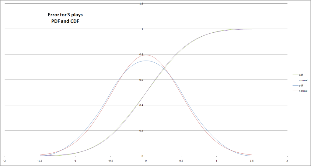
Once you get to 3 plays, the distribution of possible rounding errors starts looking very much like a normal distribution (sweet beans beluga, as my friend would say)**. Which is good, because it's probably what we would have used whether it was a good fit or not, because no one here wants to spend 8 months doing the real math.

Back to the question, how likely is it that the 990 yard rusher got rounded out of his 1000 yard season? It depends on how many carries he had, but if we know he had 300 carries, and we know 1000 yards would require a rounding error of at least 10 yards, then that is a magnitued of 2 SDs for the rounding error. That means there's only about a 2.3% chance that his precise total of 1000+ got rounded down to 990 (rule of thumb is that 95% of a normal distribution is within 2 SDs of the mean, and half of the outcomes outside of the 95% are on the low end of the distribution, leaving about two-and-a-half percent two SD above the mean). If he rushes for 999 yards (poor fellow), then there's a 42% chance he really got rounded down from 1000+. As you can see, it can make a pretty big difference over few yards, but the chances of the error being much more than that diminish pretty quickly. The same thing goes for passing yards for QBs or receivers; most of the rounding errors for a season will be within a few yards. For a 10 year career, the SD for the distribution of errors will be about 3 times as high as for a single year, so adjust accordingly if you want to look at careers (10 yards would be less than 1 SD, so that kind of error would be a lot more common at the career level).

How about if we want to know something like, what are the odds that, if we could have measured their gains with perfect precision, we would discover that Marshall Faulk actually out-gained Jim Brown? According to Pro-Football-Reference, Jim Brown rushed for 12,312 yards in 2359 carries. Marshall Faulk rushed for 12,279 yards in 2836 carries. Those numbers of carries give the distributions of rounding errors SDs of 15.4 and 14.0, respectively. We want to know how much of Faulk's distribution of possible precise totals is greater than some portion of Brown's distribution. To do this, we can subtract their individual distributions. This gives us a new distribution, which is also normal, with a mean equal to the difference between their credited yardages (33 yards) and a SD equal to the square root of the sum of the variances of their individual distributions (20.8 yards). Plug those into your calculator or spreadsheet or table of values of choice to find the odds that x < 0 (meaning the difference Brown minus Faulk is actually negative, which would indicate Faulk gained more yards than Brown), and you end up with 5.6%. Not a lot, but it's there.

Or, how about another close pairing on the all-time rushing list, Corey Dillon and O.J. Simpson? They are just 5 yards apart over a combined 5000 carries. Repeat the math, and there is a 40% chance precise measurements would give Simpson the higher total and that rounding errors pushed him below Dillon.

Really, none of this is very significant. Basically, I just dragged you through 2,000 words to tell you there's not much difference between 11,241 yards and 11,236 yards over a full career. It's common sense, really. Still, I think it's interesting to have an idea of just how little difference it makes that the NFL is so imprecise with its yardage measurements (though, to be clear, this says nothing about the additional errors that would be involved with imprecisions like eyeballing the gain and rounding it incorrectly, or the official mis-spotting the ball, or anything like that; nonetheless, you get the idea that those things are probably not that big a deal here either). At the very least, it's good to know that the rounding errors overwhelmingly fall within the range of what you would look at and say there's really not much difference there.



*I don't know if there is actually a simpler way to derive the actual distributions, just that the only way I do know how to do it is a huge pain in the ass

**Relating to last week's article on rounding errors of wOBA, deriving the actual distributions for the rounding error of wOBA is more complicated since each of the 6 terms in the wOBA formula carries a different weight, so I didn't actually go through with deriving them past 2 terms to compare to a normal distribution. Simulated results for rounding errors of wOBA do appear to fit just as well to a normal distribution, though, so you can probably use the SDs from that article as if they describe a normal distribution as well.***

***If you thought this footnote was going to be about my friend who says "sweet beans beluga", well, that's just because I didn't have a better place to insert a footnote about deriving the distribution for wOBA, so I stuck it in at a largely irrelevant spot. I can tell you, though, that she spells it balooga when she uses it as an interjection, which is kind of interesting (at least compared to footnotes about deriving distributions for possible rounding errors) Continue Reading...

ZiPS ROS Projections as Estimates of True Talent

Player projections are a great tool. They give us good, objective estimates for a player's talent going forward, which makes them useful for addressing a number of questions. For example, should your team go after Player A or Player B to play shortstop next year, and how much improvement does each expect to provide over Player C, who is already signed? How much should the team offer each if they decide to pursue them? Who is a better option to start between two players competing for a job? Did that trade your team just make make sense, and did you get an improvement in expected performance over what you had? How does the talent on my team compare to that of other teams in the division?

You can even use projections for important questions, like, who should I draft first overall in my fantasy league (I guarantee you will avoid such pitfalls as the infamous Beltran-over-Pujols,-et-al debacle, circa 2005--sorry, Uncle Jeff)?

That's all well and good for looking at the coming season, when you don't know anything about anyone's season yet, and your best guess is probably going to be heavily informed by each player's projections. However, the major problem with projections at this point in the season is that most of them are an off-season affair. They are most widely used for projecting the coming season, after all, and they can take a lot of time and computer resources to update to work mid-season and keep running over and over throughout the year.

Each player's current season performance definitely tells us a lot about how we should estimate his talent going forward, so this presents a problem with relying primarily on pre-season projections in some cases. As a result, you are more limited if you want to find projections that incorporate the current season's data to answer questions that require current estimates of talent to answer; say, for example, how does that trade my team just recently made look, or how does my team shape up for the playoffs, and how do they compare to their likely opponents, or should we give a serious look to this September call-up who's been on fire?

Fortunately, there are at least a couple freely available projections that provide in-season updates. The ones I know of are CHONE (published at Baseball Projection) and ZiPS (published at FanGraphs as ROS--rest of season--projections). Both can be good options for estimating a player's current talent level without ignoring information from his performance this season.

Because ZiPS is updated daily (as opposed to the updates every month or so that CHONE provides) and because it is now published at and frequently used by writers for the prominent stat website FanGraphs, it has become a favourite for a lot of fans for estimating current offensive talent for players. While it is great that such a tool is available and that it is used in an attempt to form objective, informed opinions, there is a serious caveat with using the current ZiPS projections on FanGraphs as true talent estimates this late in the season.

To illustrate, consider Ryan Ludwick's ZiPS ROS wOBA projection. Right now, it is .375. Before the season started, ZiPS had Ludwick pegged for a .372 wOBA. He has since aged a bit, posted a .334 figure for the year, and moved to a worse park for hitters. How did his projection go up? What is even more confusing, if you track the projections from day to day, is that yesterday, his wOBA projection was at .390 or so. The day before, it was at .385. And, if you really want to wake up in Wonderland, check the ROS projections during the last week or so of the season, when you have 8 dozen guys projected for the same .250 (or whatever it ends up being) wOBA. What is going on?

The issue is that the ZiPS ROS projections on FanGraphs are not, in fact, an estimate of the player's true talent going forward. Rather, the projection gives its best estimate, in whole numbers, for the player's number of singles, doubles, triples, homers, walks, and HBP for the rest of the season, and then FanGraphs figures out what the player's wOBA would be over the rest of the season if he hit each of those figures on the nose. For Ludwick, that means his .375 wOBA projection is not his projected talent level, but the wOBA for the following projected line:

	1B	2B	3B	HR	BB	HBP	PA	appr. wOBA
Ludwick	8	3	0	3	4	1	55	0.375

But remember that each of those components is rounded to the nearest whole number. His projected singles total could be anything from 7.5-8.5. Rounding to the nearest whole number eliminates precision, and when you have a wOBA figure that needs to go to 3 decimal places, that loss of precision can affect the projected wOBA. To see just how much difference this can make, let's pretend all of Ludwick's actual projected components are really .5 lower than the rounded off whole number (the lowest his actual projected wOBA could be), and then pretend they are all really .5 higher (the highest his actual projected wOBA could be), and see how much that affects his projected wOBA:

	1B	2B	3B	HR	BB	HBP	PA	appr. wOBA
min	7.5	2.5	0	2.5	3.5	0.5	55	0.324
max	8.5	3.5	0.5	3.5	4.5	1.5	55	0.440

As you can see, given Ludwick's projections over 55 PA, his actual projected wOBA could theoretically be anywhere from .324 to .440. That is a huge range. Of course, to be close to the extremes of the range, every component would have to be rounded in the same direction by a large amount, so it is more likely to be close to .375 than to .324 or .440.

How much more likely? To answer that, we have to know something about the distribution of possible true projected wOBAs for Ludwick, given that FanGraphs is displaying a .375 projection over 55 PA. We can do that by finding the standard deviation of the difference between actual projected wOBA and the rounded wOBA projections displayed on FanGraphs for hitters with 55 projected PA.

The actual projected total for each component, before rounding, can be anywhere from .5 less to .5 more than the rounded total. We have no idea where in that range it falls. If Ludwick is projected for 8 singles over 55 PA, it is probably close to equally likely that his true projected rate of singles per PA is 7.5 as it is 8.5, with everything in between being pretty much equally likely. This is a uniform distribution. The standard deviation for this distribution is .5/sqrt(3)=.289. That means the standard deviation for the difference between Ludwick's projected 1B total without rounding and his projected 1B total rounded to the nearest whole number is .289 singles. This describes the error in the rounded total FanGraphs displays.

Since the possible error for every component has the same uniform distribution from -.5 to .5 (except triples, since the rounded estimate of 0 can't have been rounded up, but we'll ignore that for now), the standard deviation for the error of each component is the same .289. Next, we need to know what that means in terms of affecting wOBA. The formula for wOBA is:

(0.72xNIBB + 0.75xHBP + 0.90x1B + 0.92xRBOE + 1.24x2B + 1.56x3B + 1.95xHR) / PA

That means each walk (non-intentional walk, but ZiPS doesn't differentiate, so we'll just use BB) is worth .72 in the numerator of wOBA, each HBP is worth .75, etc. The standard deviation for the error in walk total is .289, so the standard deviation of the effect of that error on the numerator of wOBA is .72*.289 (in other words, the value of each walk times the number of walks). The same process goes for each component. The following table shows the standard deviation and variance for the value of each component to the numerator:

	error	Val	StD Val	Var Val
1B	0.289	0.9	0.260	0.068
2B	0.289	1.24	0.358	0.128
3B	0.289	1.56	0.450	0.203
HR	0.289	1.95	0.563	0.317
BB	0.289	0.72	0.208	0.043
HBP	0.289	0.75	0.217	0.047
combined			0.897	0.805

The combined row shows the total variance and standard deviation for the combined rounding errors. This is simply the sum of the individual variances, with the standard deviation being the square root of that. This is what we are interested in.

.897 is not the standard deviation of wOBA itself, just the numerator. To get the standard deviation for the rounding error of wOBA, we have to divide by the numerator, which, as the above formula shows, is just PA. Ludwick is projected for 55 PA, so divide .897 by 55:

.897/55 = .016

For players projected for 55 remaining PA on FanGraphs, the standard deviation of the difference between their actual projected wOBAs and the rounded off projections which is displayed is .016. If Ludwick's actual projected wOBA is .359, that would put the rounding error in his displayed projection at one standard deviation, which would be a pretty typical observation. Of course, we don't know what anyone's actual projected wOBA is or whether the displayed figure is rounded high or low, just how imprecise the displayed figure is. In some cases, like Ludwick's, we can make a reasonable guess that the projection is rounded in a certain direction based on what we know about how projections work (i.e., a 31-32 year old with a down year probably isn't raising his projection), but all we can do is make reasonable estimates and acknowledge the limitations the imprecision imposes.

What does this mean about the value of ZiPS ROS projections? It depends on how precise you need to be. The precision drops quickly near the end of the year, but earlier in the year, they can work as good estimates of current talent. To determine how much rounding error you can expect in a projection, just divide .897 by the projected PA total for the rest of the season, and that will give you the standard deviation of the error. For example, with 200 PA projected for the ROS, the SD of the error is .897/200=.004, which is a lot more reasonable. At 20 PA, you get .045, at which point you basically can't estimate the difference between anyone with much certainty.

As a result, extrapolating the projections over longer periods of time becomes problematic. For example, if you want to compare players for next season, or to measure the magnitude of the difference between them on a full season scale (i.e., Player A is projected to be worth 30 more runs a year on offense than Player B), you are going to be multiplying the large error in wOBA over a large number of PA. Basically, you can't use them to get an idea of large-scale value.

What they are good for, however, is getting a good guess at expected production over the handful of remaining PAs this season. For example, if you want to scour your fantasy league waiver wire and see what everyone is likely to give you over the rest of the season, or if you want to evaluate a fantasy trade proposal, or whatever, then ZiPS ROS projections are great. The key to using them is, do you need a precise measure of value, and do you need to extrapolate over a large number of PAs? Anything where you are looking for true talent going forward beyond just what to expect over a handful of remaining PAs, or to discuss value in terms of a full season, you'd want to shy away from ZiPS ROS projections more and more the later in the year you get. For applications where you don't care about precision or how the projection extrapolates beyond the remaining 50 or 20 or however many PAs, and you don't need to be able to necessarily pick up differences between players with much certainty, then ZiPS ROS projections are fine.
Continue Reading...