Rounding Errors, Part II (Yardage Gains in the NFL)

Last week, I wrote about measuring the effects of rounding errors. When I was working on that article, it reminded me of a question I had been wanting to look into some time ago and then forgotten about. I had gotten to thinking about how yardage gains are measured in American football, always in full-yard increments. No matter the gain, it is always recorded to the nearest full yard (i.e. a 4-yard gain or a 5-yard gain, but never a 4.5 yard gain). What I had wondered was, if a player has a few hundred plays over a season, or a few thousand over a career, how much rounding error is involved? What are the chances that a back who rushes for 990 yards in a season really gained 1000 without rounding off his individual plays, or that a passer who threw for 3010 only reached the 3000 milestone with the aid of rounding up?

I never really thought about it enough to actually sit down and figure it out at the time, but, conveniently enough, last week's installment left us fully equipped to address this type of question. We learned then that rounding errors can be thought of in terms of continuous distributions, and that when those errors are added, the resulting distribution can be described in terms of the total combined variance and standard deviation. For the rounding errors for the yardage of football plays, we can think of this distribution as a one-yard wide distribution centered on the whole number.

In other words, let's say Barry Sanders rushes for 2 yards. Whether he really gained 4 1/2 feet, or 7 1/2 feet, or anywhere in between, the NFL is just going to call it 6 feet. That 2-yard gain could fall anywhere on the continuous spectrum from 1.5 yards to 2.5 yards, and when we see a 2-yard gain recorded in the data, we have no idea where in that spectrum the gain falls. That is a continuous distribution, and the standard deviation for the rounding error of this play is .289 yards.

Before we go on, I'd like to highlight some of the assumptions we are making here when we choose a continuous distribution that is one-yard wide. One, we are assuming every gain is properly rounded to the nearest whole yard. In reality, maybe the ref spots the ball 4.4 yards from the line of scrimmage and the scorer eyeballs that and sees it as a 5 yard gain, or the ball is spotted for a 4.6 yard gain and the scorer marks it as a 4 yard gain. Because of this, when you see a two yard gain, the distribution of possible gains will actually be a bit wider than 1 yard, and it won't be continuous, but slope downward toward the ends. However, we'll ignore that so that we can mathematically describe the situation. Another thing being ignored is the distribution of gains on all plays in the NFL, or for a given player. If more runs go for 2 yards than 1 yard, and more runs go for 3 runs than 2 yards (I am making this up; I have no idea if this is how rushing gains are distributed in the NFL or not), then when you see a 2-yard gain, it is more likely to be rounded down than rounded up. That won't give us a continuous distribution either. But, for our purposes, we are going to assume we know nothing about how gains are distributed (hey, I actually don't know that!) and act under the assumption that there is no reason to believe any number in the spectrum from 1.5 yards to 2.5 yards is any more likely than another.

Now that that is out of the way, let's continue. The SD for the rounding error of each play is .289 yards. Now, let's say Barry Sanders rushes again, this time for no gain. His total yardage is 2 yards, and the standard deviation for the rounding error is sqrt(.289^2+.289^2) = .408 yards. This is just after 2 runs, and the error is already close to half a yard and growing quickly. Is this going to be a problem as the number of plays adds up? It's still just third down, so Barry has one more play before Detroit has to punt, so let's keep going.

For his third run, Barry rushes for 87 yards. Now his total for 3 plays is 89 yards, with a standard deviation of sqrt(.289^2+.289^2+.289^2) = .500 yards. At one play, the error started out at .289. With the next play, it rose to .408, for an additional .120 yards of error (heh, look at those rounding errors popping up again). On the third run, the error rose by another .092 yards. As you can see, the effect of each additional play diminishes, so maybe it won't be much of a problem after all.

If you read last week's article, you'll remember that the rounding errors were a relatively large issue when PAs were small, but that the error shrunk substantially when PAs became high. The error in yardage we're talking about here won't ever shrink (the only reason the error shrank when we were talking about wOBA was that we divided the error by PA, and the PA term started growing a lot faster than the error term), but its growth will slow down considerably.

Instead of just 3 rushes, let's say Barry Sanders carries the ball 300 times in a season. The standard deviation of the rounding error is sqrt(300*.289^2) = 5 yards. While it only took 3 plays for the error to reach a SD of .5 yards, it took 300 plays to get up to 5 yards. If we look at Barry Sanders whole career of 3000 or so rushes, the SD of the rounding error only gets up to about 16 yards. If some QB goes all Brett Favre on us and keeps slinging the ball every which way until he racks up 6,000 completions (you only need to look at completions for QBs, since the error around the 0 yards for an incompletion can be considered to be 0, spotting errors aside), the SD on the error would still be well under 25 yards. That's pretty reassuring to the way the NFL adds things up.

There still is some imprecision from the rounding, though, so what about the questions introduced in the first paragraph? If a back is credited with 990 yards rushing, what are the chances he was above 1000 without rounding? To answer this, we need to know a little more about the distribution of possible errors. Specifically, we need to know what kind of shape the distribution takes.

If we're lucky, the distribution will be normal, because then the math is simple (or rather, there are plenty of tools readily available that do the math for us, which is a really simple way to "do" math). Remember that we started off with a uniform distribution when we only have one play, which looks like this:


That is clearly not a normal distribution, but the math is still simple with a uniform distribution. When we add a second play, then the distribution for the combined error becomes triangular:


The tip looks a bit rounded in that graph because of how Excel decided to handle things and because I am too lazy to fire up R, but it isn't. It's just straight up triangular. Again, clearly not normal, but still simple enough.

When you add in a third play, then the math for the actual distribution starts to get complicated. It is basically a piecemeal series of polynomial functions that each describe one portion of the distribution. To describe the distribution for combined rounding error for 3 plays, you need 3 different functions, and each play you add means you need to add another function to the mix. What's more, to get the distribution for 3 plays, you need to know the distribution for 2 plays. To derive the distribution for 300 plays, you have to derive the previous 299 distributions as well*, which involves thousands of individual functions. Let's just say, we really don't want to have to use the actual distributions, so we'd better hope that there is a simpler distribution that is a good approximation.

Lo and behold, there is. Here is the actual distribution for 3 plays, along with the normal approximation of the distribution using the same standard deviation:


And here is the actual CDF compared to the normal approximation (click for a larger image, since it is hard to see the difference between the two lines on this graph),


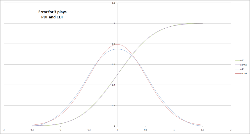
Once you get to 3 plays, the distribution of possible rounding errors starts looking very much like a normal distribution (sweet beans beluga, as my friend would say)**. Which is good, because it's probably what we would have used whether it was a good fit or not, because no one here wants to spend 8 months doing the real math.

Back to the question, how likely is it that the 990 yard rusher got rounded out of his 1000 yard season? It depends on how many carries he had, but if we know he had 300 carries, and we know 1000 yards would require a rounding error of at least 10 yards, then that is a magnitued of 2 SDs for the rounding error. That means there's only about a 2.3% chance that his precise total of 1000+ got rounded down to 990 (rule of thumb is that 95% of a normal distribution is within 2 SDs of the mean, and half of the outcomes outside of the 95% are on the low end of the distribution, leaving about two-and-a-half percent two SD above the mean). If he rushes for 999 yards (poor fellow), then there's a 42% chance he really got rounded down from 1000+. As you can see, it can make a pretty big difference over few yards, but the chances of the error being much more than that diminish pretty quickly. The same thing goes for passing yards for QBs or receivers; most of the rounding errors for a season will be within a few yards. For a 10 year career, the SD for the distribution of errors will be about 3 times as high as for a single year, so adjust accordingly if you want to look at careers (10 yards would be less than 1 SD, so that kind of error would be a lot more common at the career level).

How about if we want to know something like, what are the odds that, if we could have measured their gains with perfect precision, we would discover that Marshall Faulk actually out-gained Jim Brown? According to Pro-Football-Reference, Jim Brown rushed for 12,312 yards in 2359 carries. Marshall Faulk rushed for 12,279 yards in 2836 carries. Those numbers of carries give the distributions of rounding errors SDs of 15.4 and 14.0, respectively. We want to know how much of Faulk's distribution of possible precise totals is greater than some portion of Brown's distribution. To do this, we can subtract their individual distributions. This gives us a new distribution, which is also normal, with a mean equal to the difference between their credited yardages (33 yards) and a SD equal to the square root of the sum of the variances of their individual distributions (20.8 yards). Plug those into your calculator or spreadsheet or table of values of choice to find the odds that x < 0 (meaning the difference Brown minus Faulk is actually negative, which would indicate Faulk gained more yards than Brown), and you end up with 5.6%. Not a lot, but it's there.

Or, how about another close pairing on the all-time rushing list, Corey Dillon and O.J. Simpson? They are just 5 yards apart over a combined 5000 carries. Repeat the math, and there is a 40% chance precise measurements would give Simpson the higher total and that rounding errors pushed him below Dillon.

Really, none of this is very significant. Basically, I just dragged you through 2,000 words to tell you there's not much difference between 11,241 yards and 11,236 yards over a full career. It's common sense, really. Still, I think it's interesting to have an idea of just how little difference it makes that the NFL is so imprecise with its yardage measurements (though, to be clear, this says nothing about the additional errors that would be involved with imprecisions like eyeballing the gain and rounding it incorrectly, or the official mis-spotting the ball, or anything like that; nonetheless, you get the idea that those things are probably not that big a deal here either). At the very least, it's good to know that the rounding errors overwhelmingly fall within the range of what you would look at and say there's really not much difference there.


*I don't know if there is actually a simpler way to derive the actual distributions, just that the only way I do know how to do it is a huge pain in the ass

**Relating to last week's article on rounding errors of wOBA, deriving the actual distributions for the rounding error of wOBA is more complicated since each of the 6 terms in the wOBA formula carries a different weight, so I didn't actually go through with deriving them past 2 terms to compare to a normal distribution. Simulated results for rounding errors of wOBA do appear to fit just as well to a normal distribution, though, so you can probably use the SDs from that article as if they describe a normal distribution as well.***

***If you thought this footnote was going to be about my friend who says "sweet beans beluga", well, that's just because I didn't have a better place to insert a footnote about deriving the distribution for wOBA, so I stuck it in at a largely irrelevant spot. I can tell you, though, that she spells it balooga when she uses it as an interjection, which is kind of interesting (at least compared to footnotes about deriving distributions for possible rounding errors)
Continue Reading...

ZiPS ROS Projections as Estimates of True Talent

Player projections are a great tool. They give us good, objective estimates for a player's talent going forward, which makes them useful for addressing a number of questions. For example, should your team go after Player A or Player B to play shortstop next year, and how much improvement does each expect to provide over Player C, who is already signed? How much should the team offer each if they decide to pursue them? Who is a better option to start between two players competing for a job? Did that trade your team just make make sense, and did you get an improvement in expected performance over what you had? How does the talent on my team compare to that of other teams in the division?

You can even use projections for important questions, like, who should I draft first overall in my fantasy league (I guarantee you will avoid such pitfalls as the infamous Beltran-over-Pujols,-et-al debacle, circa 2005--sorry, Uncle Jeff)?

That's all well and good for looking at the coming season, when you don't know anything about anyone's season yet, and your best guess is probably going to be heavily informed by each player's projections. However, the major problem with projections at this point in the season is that most of them are an off-season affair. They are most widely used for projecting the coming season, after all, and they can take a lot of time and computer resources to update to work mid-season and keep running over and over throughout the year.

Each player's current season performance definitely tells us a lot about how we should estimate his talent going forward, so this presents a problem with relying primarily on pre-season projections in some cases. As a result, you are more limited if you want to find projections that incorporate the current season's data to answer questions that require current estimates of talent to answer; say, for example, how does that trade my team just recently made look, or how does my team shape up for the playoffs, and how do they compare to their likely opponents, or should we give a serious look to this September call-up who's been on fire?

Fortunately, there are at least a couple freely available projections that provide in-season updates. The ones I know of are CHONE (published at Baseball Projection) and ZiPS (published at FanGraphs as ROS--rest of season--projections). Both can be good options for estimating a player's current talent level without ignoring information from his performance this season.

Because ZiPS is updated daily (as opposed to the updates every month or so that CHONE provides) and because it is now published at and frequently used by writers for the prominent stat website FanGraphs, it has become a favourite for a lot of fans for estimating current offensive talent for players. While it is great that such a tool is available and that it is used in an attempt to form objective, informed opinions, there is a serious caveat with using the current ZiPS projections on FanGraphs as true talent estimates this late in the season.

To illustrate, consider Ryan Ludwick's ZiPS ROS wOBA projection. Right now, it is .375. Before the season started, ZiPS had Ludwick pegged for a .372 wOBA. He has since aged a bit, posted a .334 figure for the year, and moved to a worse park for hitters. How did his projection go up? What is even more confusing, if you track the projections from day to day, is that yesterday, his wOBA projection was at .390 or so. The day before, it was at .385. And, if you really want to wake up in Wonderland, check the ROS projections during the last week or so of the season, when you have 8 dozen guys projected for the same .250 (or whatever it ends up being) wOBA. What is going on?

The issue is that the ZiPS ROS projections on FanGraphs are not, in fact, an estimate of the player's true talent going forward. Rather, the projection gives its best estimate, in whole numbers, for the player's number of singles, doubles, triples, homers, walks, and HBP for the rest of the season, and then FanGraphs figures out what the player's wOBA would be over the rest of the season if he hit each of those figures on the nose. For Ludwick, that means his .375 wOBA projection is not his projected talent level, but the wOBA for the following projected line:


1B 2B 3B HR BB HBP PA
appr. wOBA
Ludwick 8 3 0 3 4 1 55
0.375

But remember that each of those components is rounded to the nearest whole number. His projected singles total could be anything from 7.5-8.5. Rounding to the nearest whole number eliminates precision, and when you have a wOBA figure that needs to go to 3 decimal places, that loss of precision can affect the projected wOBA. To see just how much difference this can make, let's pretend all of Ludwick's actual projected components are really .5 lower than the rounded off whole number (the lowest his actual projected wOBA could be), and then pretend they are all really .5 higher (the highest his actual projected wOBA could be), and see how much that affects his projected wOBA:


1B 2B 3B HR BB HBP PA appr. wOBA
min
7.5 2.5 0 2.5 3.5 0.5 55 0.324
max
8.5 3.5 0.5 3.5 4.5 1.5 55 0.440


As you can see, given Ludwick's projections over 55 PA, his actual projected wOBA could theoretically be anywhere from .324 to .440. That is a huge range. Of course, to be close to the extremes of the range, every component would have to be rounded in the same direction by a large amount, so it is more likely to be close to .375 than to .324 or .440.

How much more likely? To answer that, we have to know something about the distribution of possible true projected wOBAs for Ludwick, given that FanGraphs is displaying a .375 projection over 55 PA. We can do that by finding the standard deviation of the difference between actual projected wOBA and the rounded wOBA projections displayed on FanGraphs for hitters with 55 projected PA.

The actual projected total for each component, before rounding, can be anywhere from .5 less to .5 more than the rounded total. We have no idea where in that range it falls. If Ludwick is projected for 8 singles over 55 PA, it is probably close to equally likely that his true projected rate of singles per PA is 7.5 as it is 8.5, with everything in between being pretty much equally likely. This is a uniform distribution. The standard deviation for this distribution is .5/sqrt(3)=.289. That means the standard deviation for the difference between Ludwick's projected 1B total without rounding and his projected 1B total rounded to the nearest whole number is .289 singles. This describes the error in the rounded total FanGraphs displays.

Since the possible error for every component has the same uniform distribution from -.5 to .5 (except triples, since the rounded estimate of 0 can't have been rounded up, but we'll ignore that for now), the standard deviation for the error of each component is the same .289. Next, we need to know what that means in terms of affecting wOBA. The formula for wOBA is:

(0.72xNIBB + 0.75xHBP + 0.90x1B + 0.92xRBOE + 1.24x2B + 1.56x3B + 1.95xHR) / PA

That means each walk (non-intentional walk, but ZiPS doesn't differentiate, so we'll just use BB) is worth .72 in the numerator of wOBA, each HBP is worth .75, etc. The standard deviation for the error in walk total is .289, so the standard deviation of the effect of that error on the numerator of wOBA is .72*.289 (in other words, the value of each walk times the number of walks). The same process goes for each component. The following table shows the standard deviation and variance for the value of each component to the numerator:


error Val StD Val Var Val
1B 0.289 0.9 0.260 0.068
2B 0.289 1.24 0.358 0.128
3B 0.289 1.56 0.450 0.203
HR 0.289 1.95 0.563 0.317
BB 0.289 0.72 0.208 0.043
HBP 0.289 0.75 0.217 0.047
combined
0.897 0.805


The combined row shows the total variance and standard deviation for the combined rounding errors. This is simply the sum of the individual variances, with the standard deviation being the square root of that. This is what we are interested in.

.897 is not the standard deviation of wOBA itself, just the numerator. To get the standard deviation for the rounding error of wOBA, we have to divide by the numerator, which, as the above formula shows, is just PA. Ludwick is projected for 55 PA, so divide .897 by 55:

.897/55 = .016

For players projected for 55 remaining PA on FanGraphs, the standard deviation of the difference between their actual projected wOBAs and the rounded off projections which is displayed is .016. If Ludwick's actual projected wOBA is .359, that would put the rounding error in his displayed projection at one standard deviation, which would be a pretty typical observation. Of course, we don't know what anyone's actual projected wOBA is or whether the displayed figure is rounded high or low, just how imprecise the displayed figure is. In some cases, like Ludwick's, we can make a reasonable guess that the projection is rounded in a certain direction based on what we know about how projections work (i.e., a 31-32 year old with a down year probably isn't raising his projection), but all we can do is make reasonable estimates and acknowledge the limitations the imprecision imposes.

What does this mean about the value of ZiPS ROS projections? It depends on how precise you need to be. The precision drops quickly near the end of the year, but earlier in the year, they can work as good estimates of current talent. To determine how much rounding error you can expect in a projection, just divide .897 by the projected PA total for the rest of the season, and that will give you the standard deviation of the error. For example, with 200 PA projected for the ROS, the SD of the error is .897/200=.004, which is a lot more reasonable. At 20 PA, you get .045, at which point you basically can't estimate the difference between anyone with much certainty.

As a result, extrapolating the projections over longer periods of time becomes problematic. For example, if you want to compare players for next season, or to measure the magnitude of the difference between them on a full season scale (i.e., Player A is projected to be worth 30 more runs a year on offense than Player B), you are going to be multiplying the large error in wOBA over a large number of PA. Basically, you can't use them to get an idea of large-scale value.

What they are good for, however, is getting a good guess at expected production over the handful of remaining PAs this season. For example, if you want to scour your fantasy league waiver wire and see what everyone is likely to give you over the rest of the season, or if you want to evaluate a fantasy trade proposal, or whatever, then ZiPS ROS projections are great. The key to using them is, do you need a precise measure of value, and do you need to extrapolate over a large number of PAs? Anything where you are looking for true talent going forward beyond just what to expect over a handful of remaining PAs, or to discuss value in terms of a full season, you'd want to shy away from ZiPS ROS projections more and more the later in the year you get. For applications where you don't care about precision or how the projection extrapolates beyond the remaining 50 or 20 or however many PAs, and you don't need to be able to necessarily pick up differences between players with much certainty, then ZiPS ROS projections are fine.
Continue Reading...